Mapping FFTs to a Sphere: An Unexpected Journey
Recently, my colleague Jonathan Dupuy and I, published a paper called “Concurrent Binary Trees for Large-Scale Game Components” (details here). To showcase our technique, we’ve developed and released a demo. It renders 1:1 scale planets at 250+ FPS on a PS5 grade GPU (AMD 6650 XT).
The executable demonstrates the technique on two planets that use different ways to generate the displacement data.
-
An Earth-sized water planet (let’s call it Earth)
-
A Moon-sized celestial satellite (let’s call it Moon)
For the Earth, we went with the classic multiband Philips Spectrum + Inverse FFT approach (4 bands in our case). Which in my opinion, produces good enough results for what we’re trying to achieve.
For the Moon, we used the albedo and elevation maps that the NASA provides on its website.
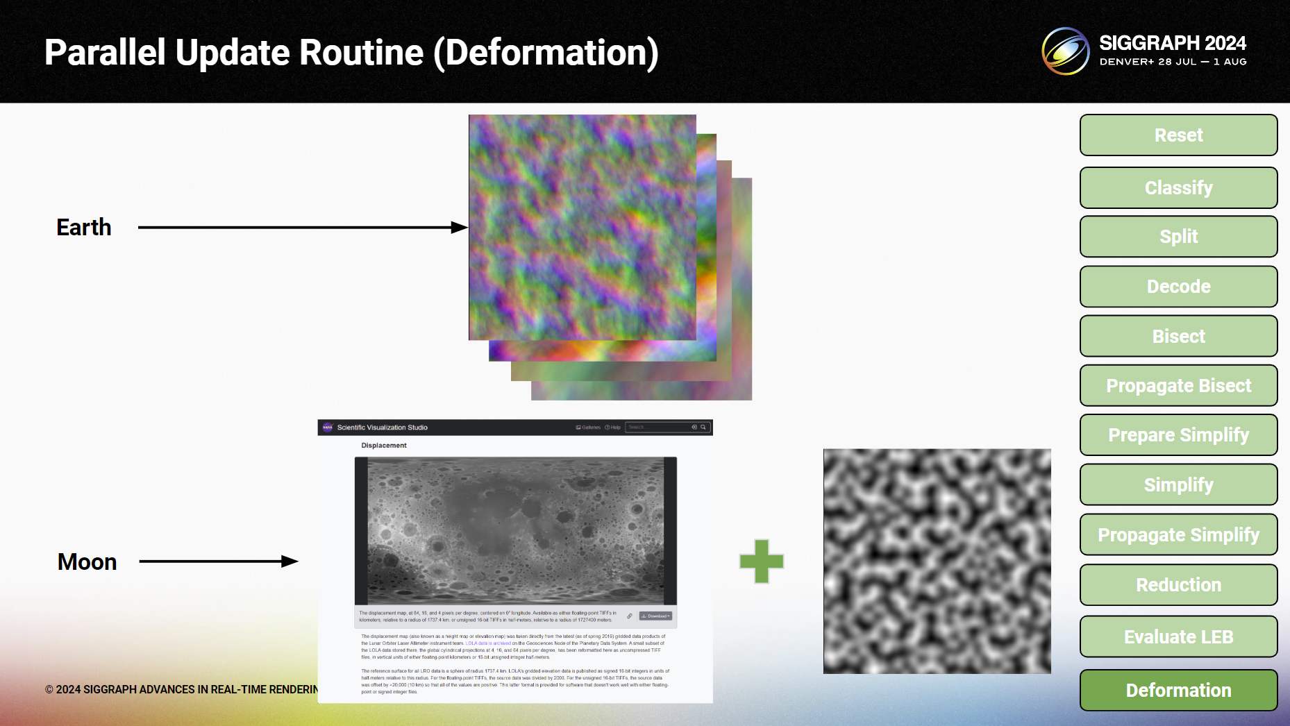 The deformation step of the update pipeline
One of the tricky things that we had to answer for rendering the Earth is the eternal: How do you map a 2D repeatable texture onto a sphere without having visible singularities?
There are many ways to do this. One is having multiple evaluations of the simulation and blending those while toning down each simulation to eventually hide the singularities. In our case (mainly for performance reasons) we wanted to have only one FFT simulation evaluation per vertex (for the displacement) and per fragment (for the normals). We already had to do 4 texture fetches per evaluation, which is quite a lot.
Long story short, the idea is to have a mapping that is mirrored around the equator while locally killing the horizontal displacement to avoid having a seam. It actually works surprisingly well.
Point projection
Longer story, we didn’t go with the classic Latitude/Longitude representation as it has two singularities (at the poles). Our starting point ended up being a function that projects each point of the surface of a sphere onto a disk.
float2 project_position_to_disk_naive(float3 posNPS)
{
    float r = acos(posNPS.y) / HALF_PI;
    float s = (posNPS.x * posNPS.x + posNPS.z * posNPS.z);
    float p = s != 0.0 ? 1.0 / sqrt(posNPS.x * posNPS.x + posNPS.z * posNPS.z) * r :  0.0;
    float up = posNPS.x * p;
    float vp = posNPS.z * p;
    return float2(up, vp);
}
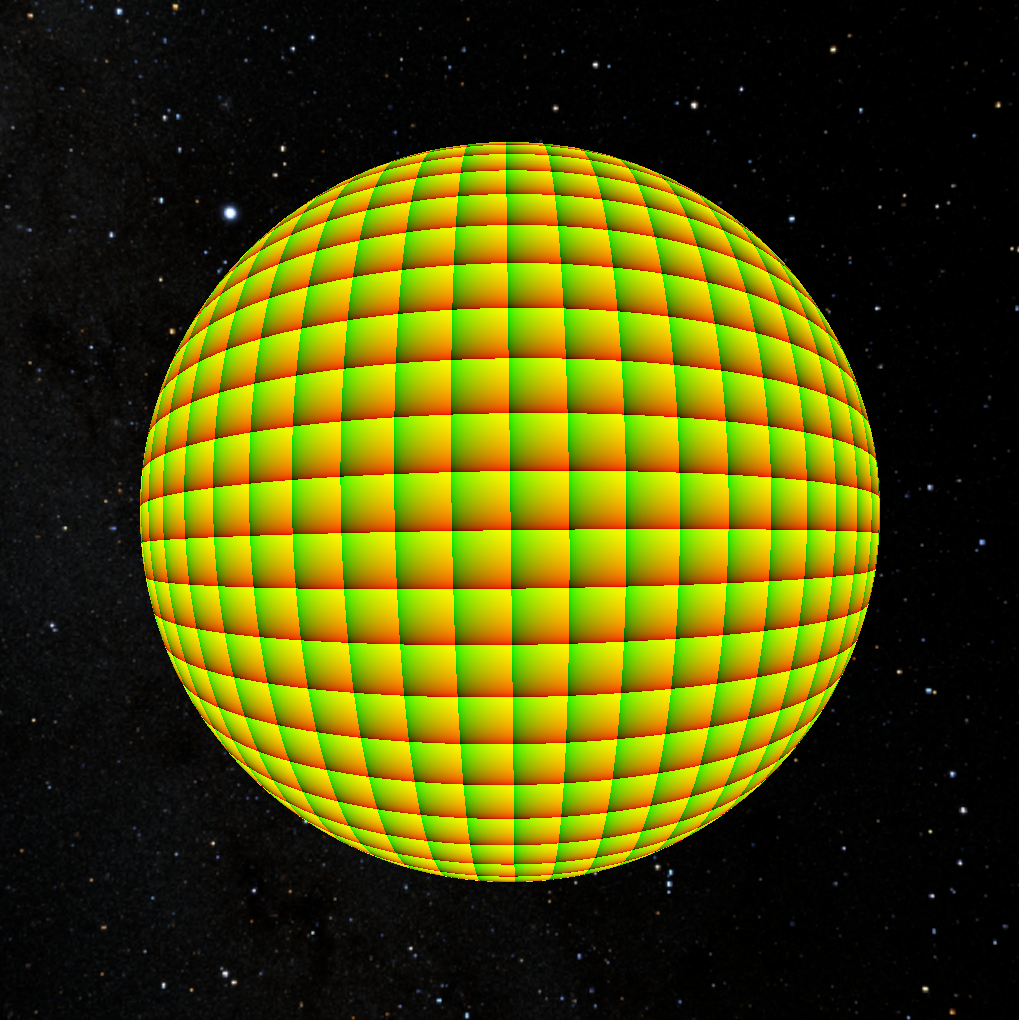 Disk projection at the north pole
This function takes as an input a normalized planet space position (NPS) (this is simply the world space position with the origin at the center of the planet divided by the radius of the planet) and returns a normalized sampling UV. At the first glance, the mapping looks quite nice from a top down view, but there are four major drawbacks:
- A massive singularity in lower part of the hemisphere
- A less and less orthogonal tangent space basis as we move away from the north pole
- Strong precision artifacts since we’re relying on the square root and trigonometric functions (and we’re operating in simple precision floating points)
- The area of each tile varies a lot which as the effect of compressing the FFT band into smaller areas
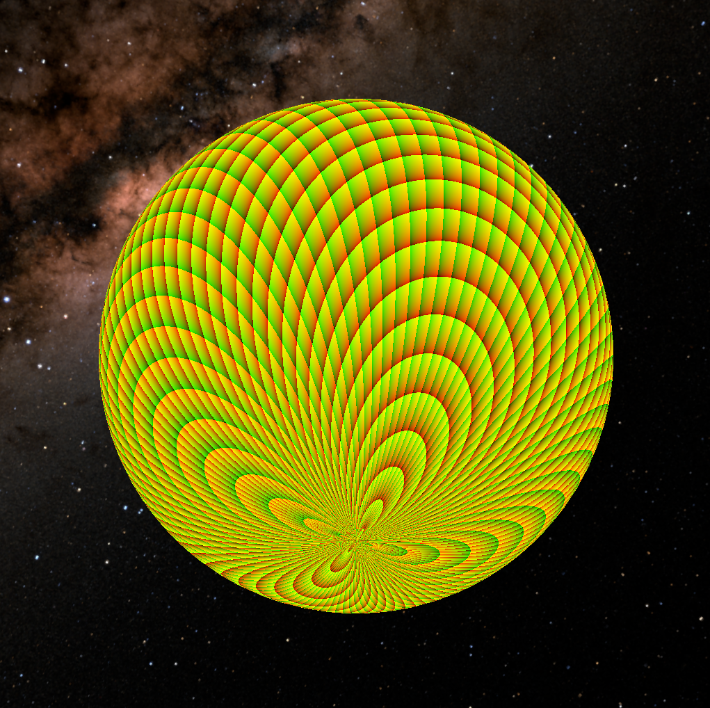 Disk projection at the south pole
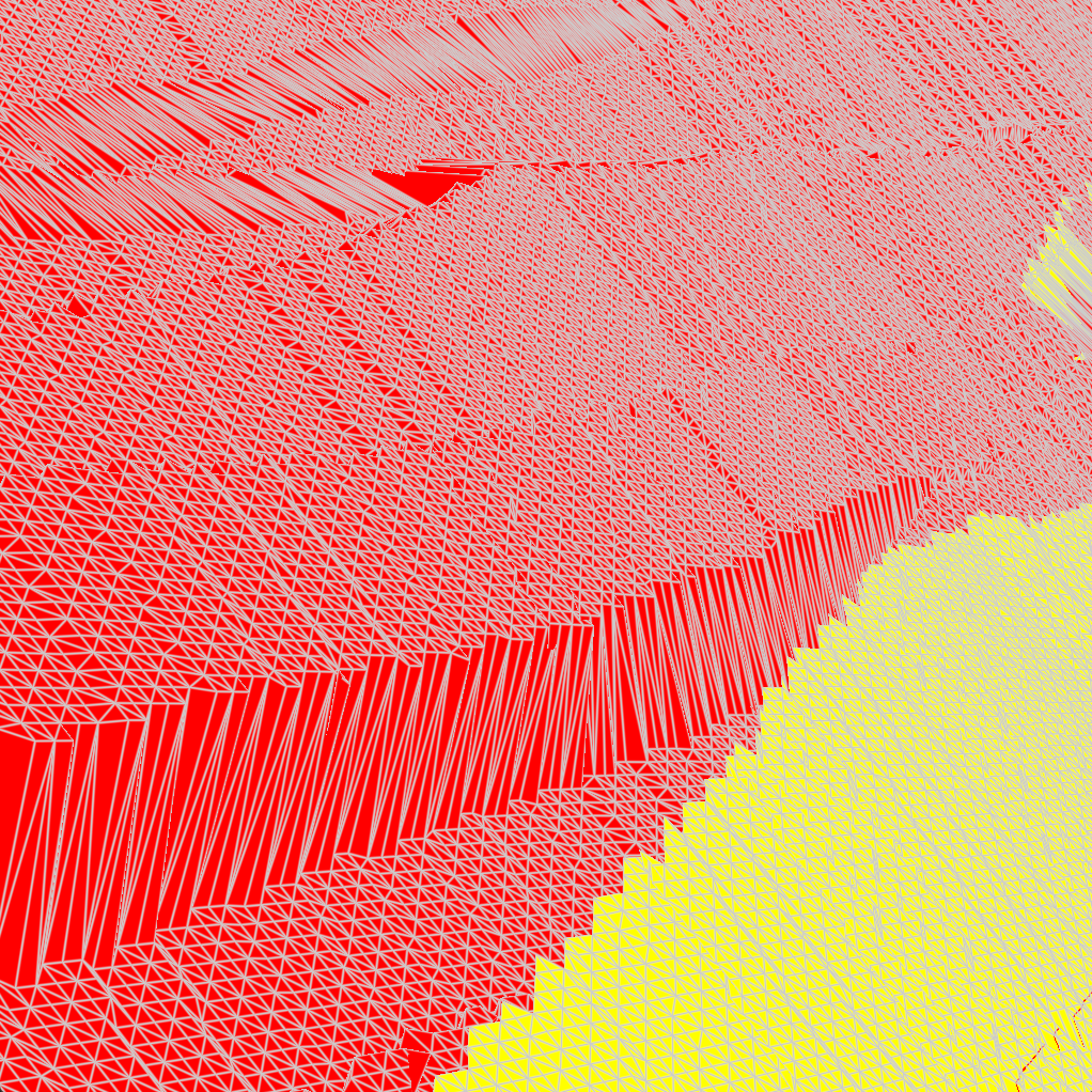 SP floating point artifacts due to the disk projection
The first step to handle these artifacts is to apply an absolute value to the y coordinate. This will mirror the pattern at the equator.
float2 project_position_to_disk_improv(float3 posNPS)
{
    float r = acos(abs(posNPS.y)) / HALF_PI;
    float s = (posNPS.x * posNPS.x + posNPS.z * posNPS.z);
    float p = s != 0.0 ? 1.0 / sqrt(posNPS.x * posNPS.x + posNPS.z * posNPS.z) * r :  0.0;
    float up = posNPS.x * p;
    float vp = posNPS.z * p;
    return float2(up, vp);
}
Doing this modification, we get something like this. Which has three benefits:
- Gets rid of the singularity
- Mitigate the orthogonality issue with the local tangent space basis
- The area of each tile is roughly the same
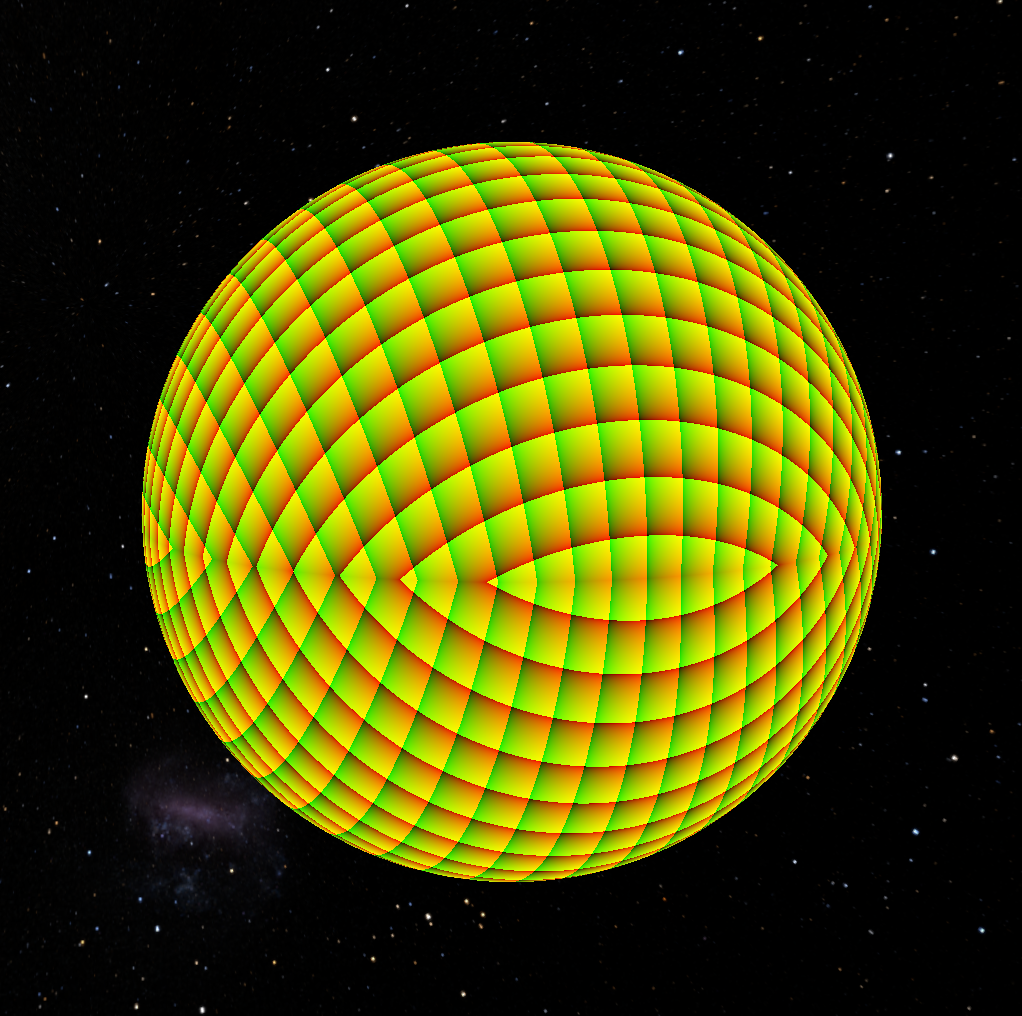
But this has a drawback, a new pattern appears at the equator. This pattern doesn’t introduce any discontinuities in the sampling coordinates, but it introduces artifacts in the final mesh.
The FFT simulation produces both vertical and horizontal displacements in the tangent space of the planet. Which when mirrored produces either stretching or overlapping artifacts on each side of the equator.
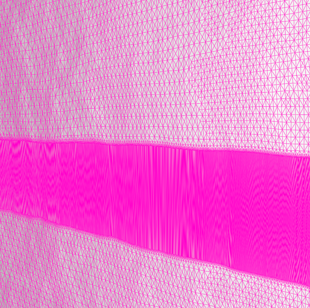 Stretching artifacts at the equator
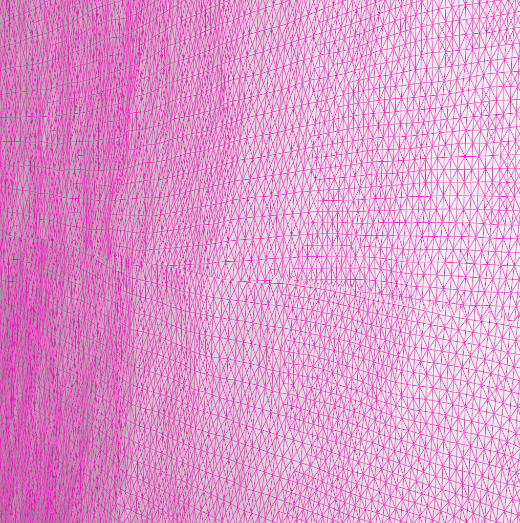 Overlapping artifacts at the equator
The next trick that we use is dampening the horizontal displacement in the neighborhood of the equator. We start this at 5km from the equator. This helps to get rid of these artifacts and already looks much better:
// Equation-reduction chopiness (5kms around the equator)
float elevation = saturate(abs(float(positionPS.y)) * 5000);

// Evaluate the displacement
float3 displacement = EvaluateDisplacement(sampleUV, elevation, distanceToCamera, _PatchSize, _Choppiness, _PatchFlags);
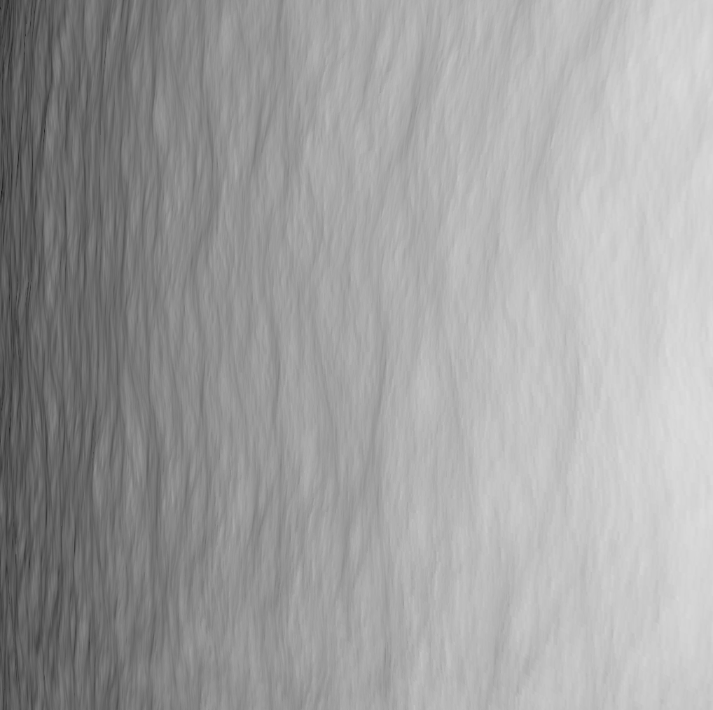 NdotV view of the geometry at the equator
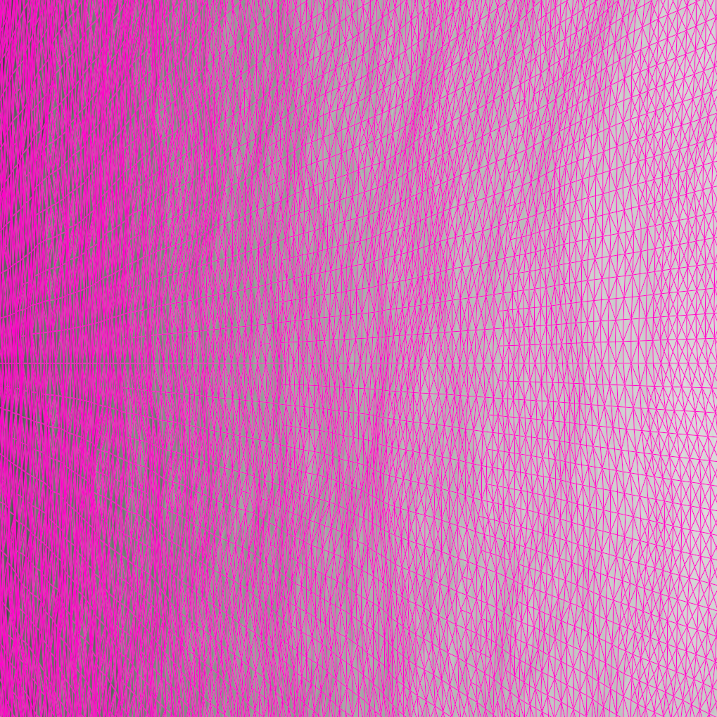 Wireframe view of the geometry at the equator
We also need to get rid of the artifacts caused by SP floats. To achieve that, we’ll be doing the projection with double precision floating points (DP floats). Thus, we need to have a double implementation of the inverse square root and of the arccos functions
- Inv_Sqrt: We start from the fast inverse square root method and make sure there are three iterations of Newton’s method to get something precise enough (otherwise we get visible artifacts)
- ArcCos: We’ve used this one found on shadertoy, but has an inconsistent behavior when we’re getting closer to zero, we had to adapt the projection routine at the northen hemisphere
double invsqrt_double(double number)
{
    double y = number;
    double x2 = y * 0.5;
    uint low, high;
    asuint(number, low, high);
    int64_t i = (int64_t(high) << 32ull) | int64_t(low);
    // The magic number is for doubles is from https://cs.uwaterloo.ca/~m32rober/rsqrt.pdf
    i = 0x5fe6eb50c7b537a9 - (i >> 1);
    y = asdouble(uint(i & 0xffffffffull), uint((i >> 32ull) & 0xffffffffull));
    y = y * (1.5 - (x2 * y * y));   // 1st iteration
    y = y * (1.5 - (x2 * y * y));   // 2nd iteration
    y = y * (1.5 - (x2 * y * y));   // 3nd iteration
    return y;
}

double acos_double(double x)
{
    double y = abs(clamp(x, -1.0, 1.0));
    double sqrtY = y != 1.0 ? sqrt_double(1.0 - y) : 0.0;
    double z = (-0.168577 * y + 1.56723) * sqrtY;
    return x > 0.0 ? z : 0.5 * PI;
}

double2 project_position_to_disk(double3 posNPS)
{
    // The acos is not viable close to the origin, we can actually use the coords straight away when we are close to the origin.
    double v = abs(posNPS.y) + 1e-10;
    if (v <= 0.999)
    {
        // Normalize the coordinates
        double r = acos_double(v) / HALF_PI;
        double s = (posNPS.x * posNPS.x + posNPS.z * posNPS.z);
        double p = s != 0.0 ? invsqrt_double(posNPS.x * posNPS.x + posNPS.z * posNPS.z) * r :  0.0;
        double u = posNPS.x * p;
        double v = posNPS.z * p;
        return double2(u, v);
    }
    return posNPS.xz / HALF_PI;
}
Sampling routine
Now, let’s talk about the sampling itself. The naïve sampling routine looks something like this:
    // Process each band
    for (uint bandIdx = 0; bandIdx < NUM_WATER_BANDS; ++bandIdx)
    {
        // Evaluate the sampling UV
        double2 bandUV = frac_double2(sampleUV / double(patchSize[bandIdx]));

        // Read the displacement
        float3 bandDis = _DisplacementBuffer.SampleLevel(displacement_buffer_sampler, float3(bandUV, bandIdx), 0, 0).xyz;

        // Distance based attenuation
        float att = lerp(1.0, 0.0, saturate((distanceToCamera - patchSize[bandIdx] * DISPLACEMENT_BAND_ATTENUATION_START) / (patchSize[bandIdx] * DISPLACEMENT_BAND_ATTENUATION_END)));

        // Apply the attenuation
        att *= (patchFlags >> bandIdx) & 0x1;
        displacement += bandDis * att;
    }

    // Swizzle the deformations
    displacement = float3(-displacement.y, displacement.x, -displacement.z);

    // Adjust the horizontal displacement
    displacement.xz *= lerp(0.0, choppiness, elevation);

    // Return the result
    return displacement;
You’ll note that we do not feed directly the sampling UVs to the SampleLevel function and that’s because the sampler fails to handle properly the repeat operation with doubles. We need to do it ourselves so we had to implement a frac_double function for that.
double floor_double(double v)
{
    double r = double(int64_t(v));
    return v < 0 ? r - 1 : r;
}

double frac_double(double v)
{
    return v - floor_double(v);
}
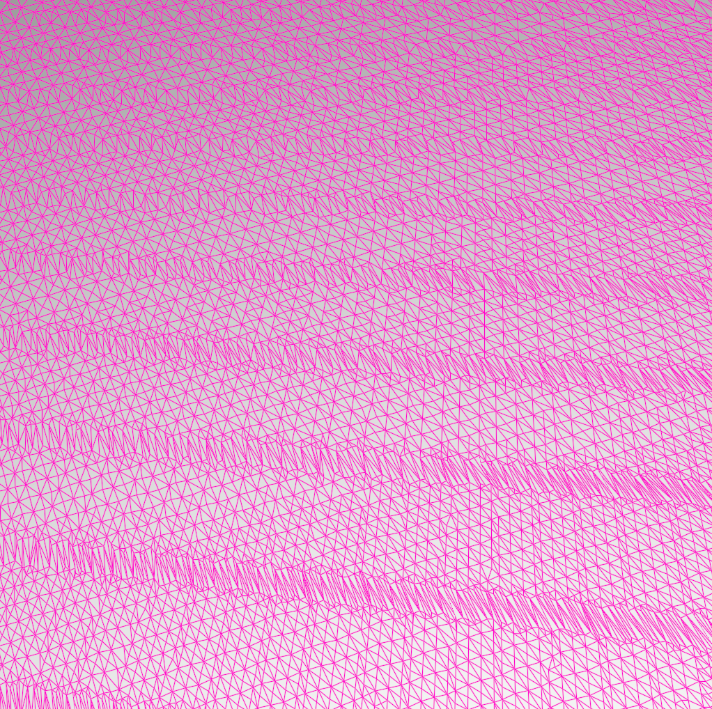 Artifacts due to the repeat pattern using the sampler
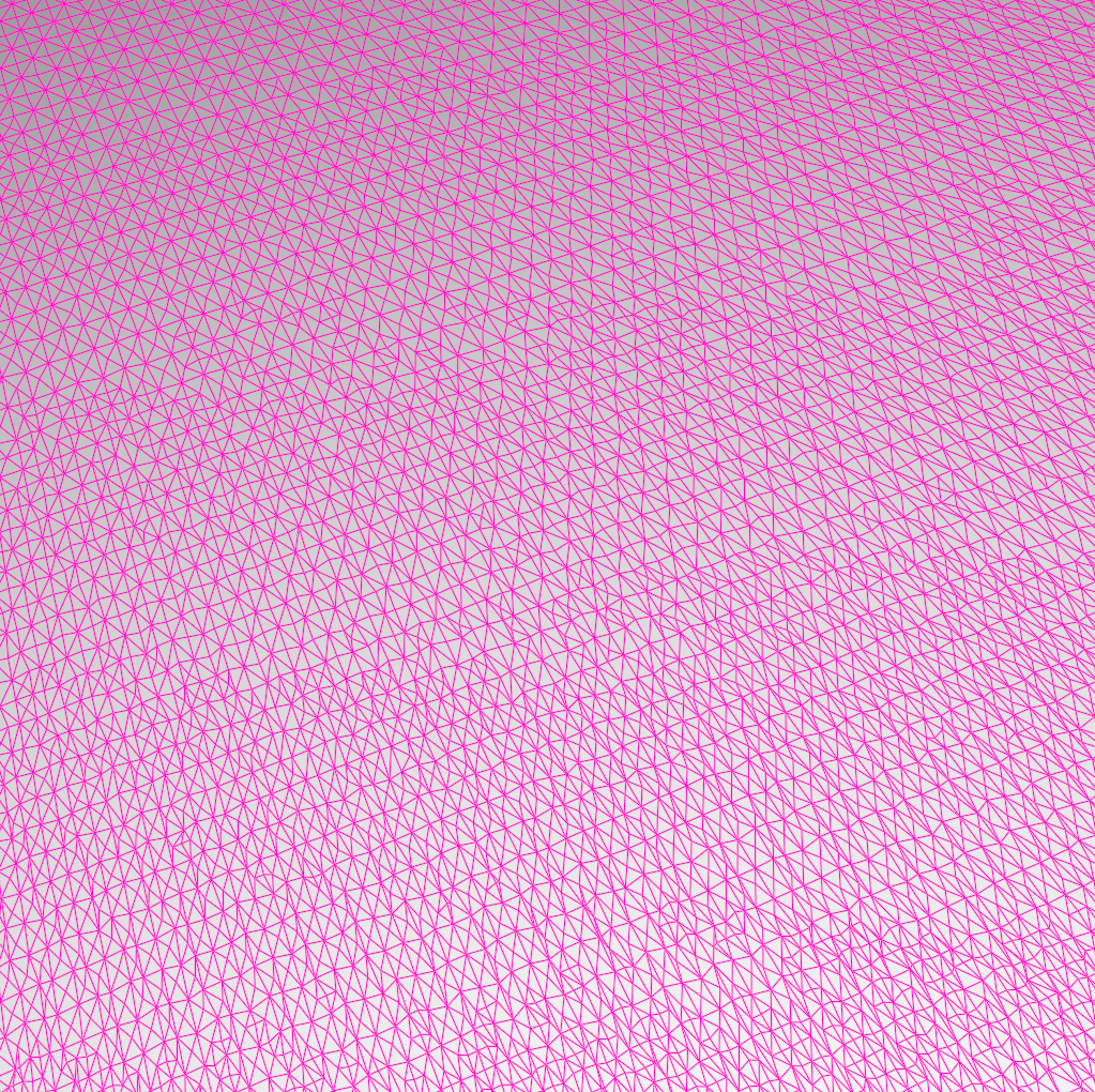 Fixed artifacts by manually doing the repeat operation
We have more artifacts due to the sampler’s discretization not handling properly the double-precision floating points (and that mainly for the larger band). To correct that, we manually do the bilinear interpolation for the band 0. Note that this artifact is less perceptible when sampling the normals, thus we don’t have to do this.
    // Evaluate the sampling UV
    double2 bandUV = frac_double2(sampleUV / double(patchSize.x));

    // For the first band, we do the bilinear interpolation manually due to interpolator float point precision issues
    double2 unnormalized = bandUV * 256;
    unnormalized.y -= 0.5;
    int2 tapCoord = (int2)floor_double2(floor_double2(unnormalized) + 0.5);

    // Read the 4 points (don't forget to wrap)
    float3 p0 = _DisplacementBuffer.Load(int4((tapCoord) & (256 - 1), 0, 0)).xyz;
    float3 p1 = _DisplacementBuffer.Load(int4((tapCoord + int2(1, 0)) & (256 - 1), 0, 0)).xyz;
    float3 p2 = _DisplacementBuffer.Load(int4((tapCoord + int2(0, 1)) & (256 - 1), 0, 0)).xyz;
    float3 p3 = _DisplacementBuffer.Load(int4((tapCoord + int2(1, 1)) & (256 - 1), 0, 0)).xyz;

    // Do the bilinear interpolation
    float2 fraction = float2(frac_double2(unnormalized));
    float3 i0 = lerp(p0, p1, fraction.x);
    float3 i1 = lerp(p2, p3, fraction.x);
    displacement = lerp(i0, i1, fraction.y);
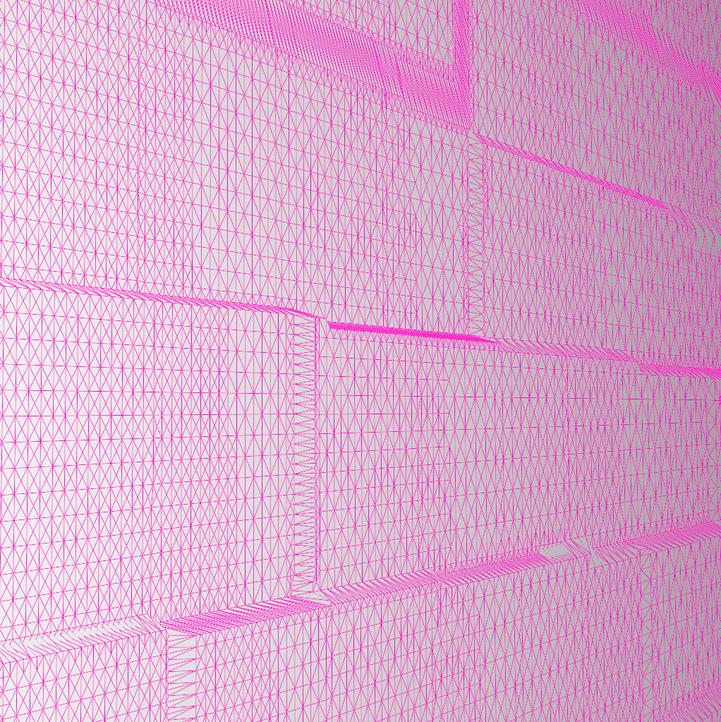 Artifacts due to the sampler for the band 0
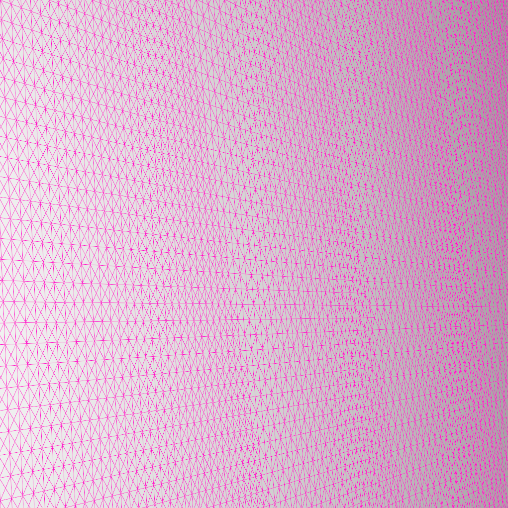 Fixed sampling for the band 0
The next step is to build a local tagent space that will be used for applying the displacement and normal disturbance. After deriving our parametrization, here is the corresponding code:
float3x3 get_local_frame(float3 posNPS, float2 uv)
{
    // In case we are close to the origin, we don't need to evaluate the local frame
    float u2 = uv.x * uv.x;
    float v2 = uv.y * uv.y;
    float u2v2 = u2 + v2;
    float sqrt_u2v2 = sqrt(u2 + v2);
    float u2v2_32 = (sqrt_u2v2 * u2v2);
    float T = (HALF_PI * sqrt_u2v2);
    float B = T < 1e-5 ? T : sin(T);
    float A = T < 1e-5 ? 1.0 - T : cos(T);

    // Tangent
    float tu_x = PI * u2 * A / (2 * u2v2) + v2 * B / u2v2_32;
    float tu_y = -PI * uv.x * B / (2.0 * sqrt_u2v2);
    float tu_z = 0.5 * uv.x * uv.y * (PI * A / u2v2 - 2.0 * B / u2v2_32);

    // Bitangent
    float btv_x = 0.5 * uv.x * uv.y * (PI * A / u2v2 - 2.0 * B / u2v2_32);
    float btv_y = -PI * uv.y * B / (2.0 * sqrt_u2v2);
    float btv_z = PI * v2 * A / (2 * u2v2) + u2 * B / u2v2_32;

    // Normalize the results
    float3 tang, bitang;
    if (abs(uv.x) >= 1e-7)
        tang = normalize(float3(tu_x, tu_y, tu_z));
    else
        tang = float3(1, 0, 0);

    if (abs(uv.y) >= 1e-7)
        bitang = normalize(float3(btv_x, btv_y, btv_z));
    else
        bitang = float3(0, 0, 1);

    // Flip operation in case we are in the lower hemisphere
    if (posNPS.y < 0.0)
    {
        tang.y = -tang.y;
        bitang.y = -bitang.y;
    }

    // return the basis
    return float3x3(tang, posNPS, bitang);
}
Now let’s move to the normal evaluation. We use the same parametrization as for the displacement, but as you can see in the next screenshots we have a line artifact at the center of the image (left) and that is due to the sampler failing to do properly the mip selection.
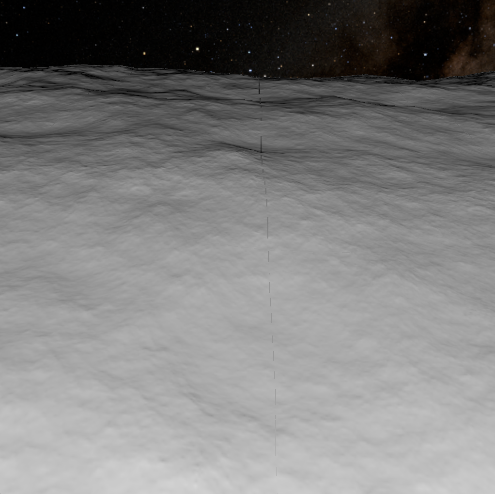 Artifacts due to the sampler mip selection routine
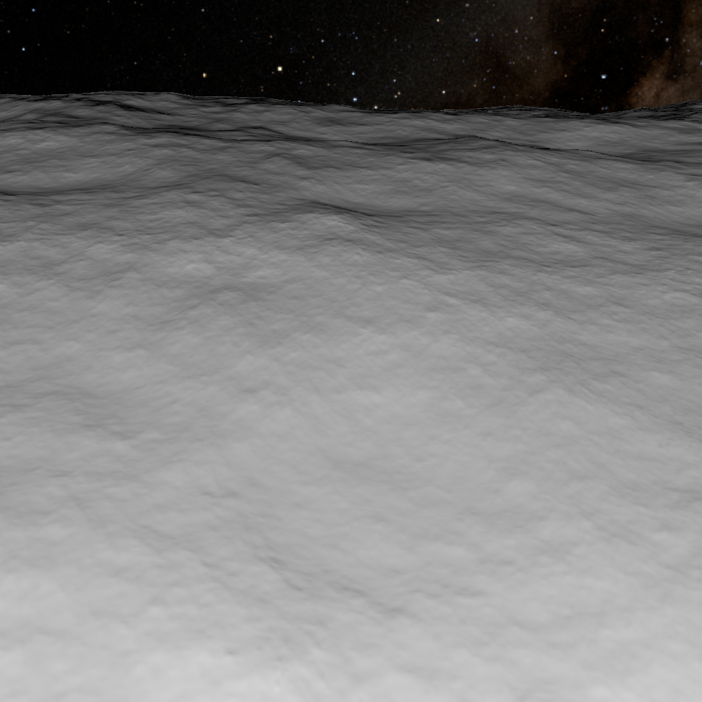 Fixed mip selection routine
To correct this artifact, the same way we do it for the displacement, we have to manually do the repeat operation. On top of that, we need to handle the mip selection and feed that as an input to the SampleGrad function. Given that we have to do the frac ourselves, we cannot naïvely use the ddx/ddy function to have the per pixel-gradients (functions that do not support doubles). We need to have a routine to adjust the gradient depending what was the result of the frac for the neighboring worker threads.
Depending on the render path, we need to take advantage of either the helper lane derivatives or the compute shader derivatives that were added in SM 6.6.
float pick_closest(float p, float n, float s)
{
    float nC = n + s;
    float distX0 = p - n;
    float distX1 = p - nC;
    return abs(distX0) < abs(distX1) ? n : nC;
}

float2 compare_and_pick(float2 p, float2 n, float s)
{
    return float2(pick_closest(p.x, n.x, s), pick_closest(p.y, n.y, s));
}

void evaluate_frac_derivatives(float2 bandUV, out float2 uvDDX, out float2 uvDDY)
{
    // Evaluate the derivatives
    float2 ddxUV = ddx(bandUV);
    float2 uvX = bandUV + ddxUV;
    uvX = compare_and_pick(bandUV, uvX, 1.0);
    uvX = compare_and_pick(bandUV, uvX, -1.0);
    uvDDX = bandUV - uvX;

    float2 ddyUV = ddy(bandUV);
    float2 uvY = bandUV + ddyUV;
    uvY = compare_and_pick(bandUV, uvY, 1.0);
    uvY = compare_and_pick(bandUV, uvY, -1.0);
    uvDDY = bandUV - uvY;
}

// Compute the UV coord
float2 bandUV = float2(frac_double2(sampleUV / patchSize[bandIdx]));

// Evaluate the derivatives for the sampling
float2 uvDDX, uvDDY;
evaluate_frac_derivatives(bandUV, uvDDX, uvDDY);

// Sample the surface gradients
float3 bandSG = _SurfaceGradientTexture.SampleGrad(surface_gradient_texture_sampler, float3(bandUV, bandIdx), uvDDX, uvDDY, 0).xyz;
Fun fact: In our demo, we’ve used the surface gradient framework to represent and combine the normals.
And with that, we can achieve an artifact-free projection and sampling of our 4 FFT bands on the geometry generated by the technique presented in our paper.
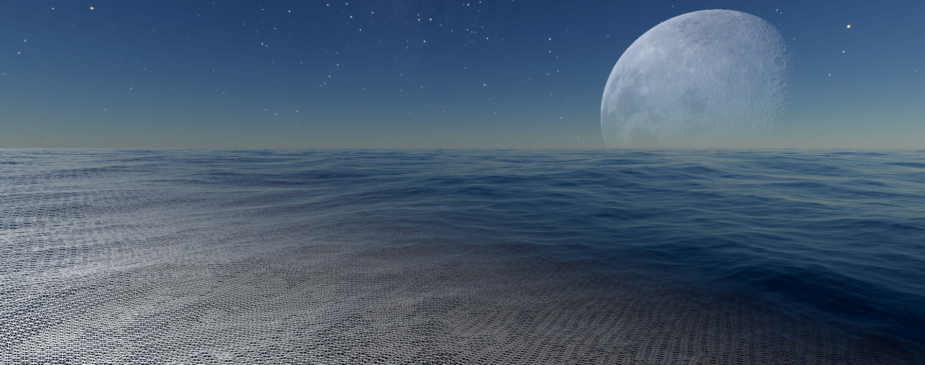 Camera above the water surface
For more details, I invite you to check the demo source code that you can find in this github repo.